
Stochastic Gradient Descent (SGD) is a fundamental optimization algorithm that has become the backbone of modern machine learning, particularly in training deep neural networks. Let's dive deep into how it works, its advantages, and why it's so widely used.
The Core Concept
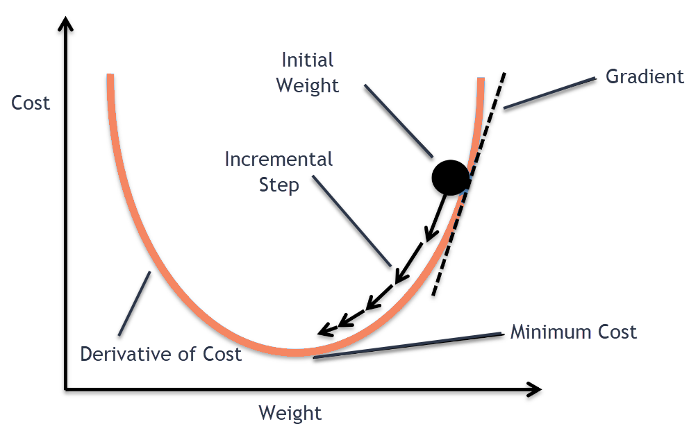
At its heart, SGD is an optimization technique that helps find the minimum of a function - specifically, the function that represents the error or loss in a machine learning model. Instead of calculating the gradient using the entire dataset (as in traditional gradient descent), SGD approximates it using a small random sample of data points.
How SGD Works
The algorithm follows these key steps:
- Random Sampling: Select a small random batch of training examples
- Calculate Gradient: Compute the gradient (direction of steepest descent) for this batch
- Update Parameters: Adjust the model's parameters in the opposite direction of the gradient
- Repeat: Continue this process until convergence or a stopping criterion is met
The mathematical update rule can be expressed as: θ = θ - η ∇J(θ; x(i), y(i))
Where:
- θ represents the model parameters
- η (eta) is the learning rate
- ∇J represents the gradient of the loss function
- x(i) and y(i) are the input and target output for the current sample
Implementing SDG
Basic SGD Implementation
import numpy as npclass SGD:def __init__(self, learning_rate=0.01, momentum=0.0):self.learning_rate = learning_rateself.momentum = momentumself.velocity = Nonedef update(self, params, gradients):if self.velocity is None:self.velocity = [np.zeros_like(param) for param in params]for i, (param, grad) in enumerate(zip(params, gradients)):# Update velocity with momentumself.velocity[i] = self.momentum * self.velocity[i] - self.learning_rate * grad# Update parametersparam += self.velocity[i]
The SGD class implements the Stochastic Gradient Descent optimization algorithm. The __init__ method initializes the learning rate and momentum. self.velocity is crucial for momentum; it stores the accumulated past gradients. The update method calculates the velocity using the momentum and current gradient, then updates the parameters by subtracting the velocity (scaled by the learning rate). The momentum term allows the optimizer to "roll" through the parameter space, smoothing out oscillations and potentially escaping local minima.
Linear Regression with SGD
The code below demonstrates a complete implementation of linear regression trained using mini-batch stochastic gradient descent with momentum. It covers data generation, model definition, optimization, mini-batching, and the training loop.
class LinearRegressionSGD:def __init__(self, learning_rate=0.01, momentum=0.0):self.weights = Noneself.bias = Noneself.optimizer = SGD(learning_rate, momentum)def initialize_parameters(self, n_features):self.weights = np.random.randn(n_features) * 0.01self.bias = 0def forward(self, X):return np.dot(X, self.weights) + self.biasdef compute_gradients(self, X, y, y_pred):m = len(X)dw = (1/m) * np.dot(X.T, (y_pred - y))db = (1/m) * np.sum(y_pred - y)return dw, dbdef train_step(self, X, y):# Forward passy_pred = self.forward(X)# Compute gradientsdw, db = self.compute_gradients(X, y, y_pred)# Update parameters using SGDself.optimizer.update([self.weights, self.bias], [dw, db])# Compute lossloss = np.mean((y_pred - y) ** 2)return loss
The LinearRegressionSGD class defines the linear regression model. __init__ sets up the weights, bias, and the optimizer (using the SGD class). initialize_parameters initializes the weights with small random values and the bias to zero. forward performs the linear combination of features and weights, adding the bias to produce predictions. compute_gradients calculates the gradients of the loss function with respect to the weights and bias using the mean squared error. train_step performs a single training step: it calculates predictions, computes gradients, updates parameters using the optimizer, and calculates the loss.
# Example with Mini-batch SGDdef create_mini_batches(X, y, batch_size):mini_batches = []data = np.hstack((X, y.reshape(-1, 1)))np.random.shuffle(data)n_minibatches = data.shape[0] // batch_sizefor i in range(n_minibatches):mini_batch = data[i * batch_size:(i + 1) * batch_size, :]X_mini = mini_batch[:, :-1]y_mini = mini_batch[:, -1]mini_batches.append((X_mini, y_mini))return mini_batches
The create_mini_batches function implements mini-batching. It shuffles the data and divides it into smaller batches. Mini-batching offers a compromise between the speed of batch gradient descent (using all data at once) and the noise of stochastic gradient descent (using one data point at a time). It processes a small batch of data at each step, reducing computation time compared to batch gradient descent and providing more stable updates than stochastic gradient descent.
# Example usagedef train_model():# Generate synthetic datanp.random.seed(42)X = np.random.randn(1000, 5) # 1000 samples, 5 featurestrue_weights = np.array([1, 2, 3, 4, 5])y = np.dot(X, true_weights) + np.random.randn(1000) * 0.1# Initialize modelmodel = LinearRegressionSGD(learning_rate=0.01, momentum=0.9)model.initialize_parameters(n_features=5)# Training with mini-batchesbatch_size = 32n_epochs = 100for epoch in range(n_epochs):mini_batches = create_mini_batches(X, y, batch_size)epoch_loss = 0for X_mini, y_mini in mini_batches:loss = model.train_step(X_mini, y_mini)epoch_loss += lossif (epoch + 1) % 10 == 0:print(f"Epoch {epoch + 1}, Loss: {epoch_loss/len(mini_batches):.6f}")return model
The train_model function sets up the training process. It generates synthetic data for demonstration. It initializes the LinearRegressionSGD model, creates mini-batches of the training data, and iterates through the training epochs. In each epoch, it iterates through the mini-batches, performing a training step and accumulating the loss. It prints the average loss at intervals.
# Run trainingif __name__ == "__main__":model = train_model()
The if __name__ == "__main__": block ensures the train_model function is called when the script is executed directly. This starts the training process, and the trained model is returned.
Advantages of SGD
The popularity of SGD stems from several key advantages:
- Computational Efficiency: Processing small batches is much faster than using the entire dataset, especially with large datasets that might not fit in memory.
- Noise as a Feature: The randomness in sampling can help escape local minima and find better solutions. This "noisy" optimization process can lead to more robust models.
- Online Learning: SGD can process data on-the-fly, making it suitable for streaming data and online learning scenarios.
- Memory Efficiency: Since it only needs to store and process a small batch of data at a time, SGD is memory-efficient.
Variants and Improvements
Several variations of SGD have been developed to address its limitations:
Mini-batch SGD
Instead of using single samples, mini-batch SGD uses small batches of data (typically 32-512 samples). This provides a better balance between computational efficiency and gradient estimation quality.
Momentum
Adding momentum helps SGD maintain direction and speed when moving through areas of consistent gradient, while dampening oscillations in areas of varying gradients: v = γv - η∇J(θ) θ = θ + v
Adam (Adaptive Moment Estimation)
One of the most popular SGD variants, Adam combines momentum with adaptive learning rates for each parameter. It maintains both first-order (mean) and second-order (uncentered variance) moments of the gradients.
Practical Considerations
When implementing SGD, several factors need careful consideration:
- Learning Rate Selection The learning rate η is crucial for convergence. Too large, and the algorithm may overshoot; too small, and training becomes unnecessarily slow. Many practitioners use learning rate schedules that decrease η over time.
- Batch Size Choosing the right batch size involves trading off between:
- Computational efficiency
- Memory usage
- Gradient estimation quality
- Generalization performance
- Data Shuffling Randomly shuffling the training data between epochs helps prevent the algorithm from learning unwanted patterns in the data presentation order.
- Regularization SGD works well with various regularization techniques like L1/L2 regularization and dropout, which help prevent overfitting.
Applications in Deep Learning
SGD's importance in deep learning cannot be overstated. It enables training of complex neural networks by:
- Processing massive datasets efficiently
- Handling non-convex optimization problems
- Adapting to different architectures and loss functions
- Supporting parallel and distributed training
Common Challenges and Solutions
- Vanishing/Exploding Gradients
- Solution: Proper initialization, batch normalization, and gradient clipping
- Saddle Points
- Solution: Momentum and adaptive learning rate methods help escape saddle points
- Poor Conditioning
- Solution: Second-order methods or adaptive learning rate algorithms
Best Practices
To get the most out of SGD:
- Start with a reasonable learning rate and batch size based on similar problems or guidelines.
- Monitor training metrics carefully:
- Loss value trends
- Gradient magnitudes
- Parameter updates
- Use validation data to track generalization performance and avoid overfitting.
- Consider implementing early stopping when validation metrics plateau.
Future Directions
Research in SGD continues to evolve, focusing on:
- Adaptive optimization methods
- Distributed and parallel implementations
- Theoretical understanding of generalization properties
- Application to new architectures and problem domains
More Articles from Python Central
Automating Image Handling with Integrating Depositphotos API with Python