Mastering Linear Regression in Python

Introduction to Linear Regression

Linear regression is a fundamental machine learning algorithm used for predicting a continuous target variable based on one or more predictor variables. It is a powerful and widely-used technique for modeling the linear relationship between input features and an output.

In this article, we'll dive deep into implementing linear regression in Python, covering both simple (single feature) and multiple (multi-feature) linear regression models.

Simple Linear Regression

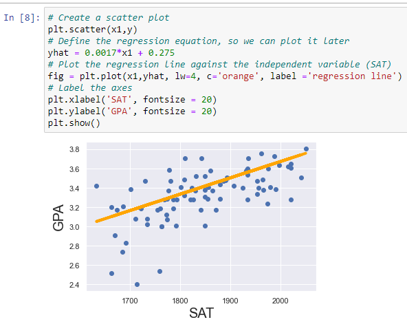
Simple linear regression is used when you have one input feature (x) and one output or target feature (y). The goal is to find the best-fit line that minimizes the sum of squared differences between the predicted values and the actual values.

The equation for a simple linear regression model is:

y = mx + b

Where:

y is the target or dependent variable
x is the predictor or independent variable
m is the slope of the line
b is the y-intercept

Example: Predicting Housing Prices

Let's look at an example of simple linear regression using the Boston Housing dataset.

import pandas as pd

from sklearn.linear_model import LinearRegression
from sklearn.model_selection import train_test_split

# Load the Boston Housing dataset
data = pd.read_csv('boston.csv')

# Define the input (feature) and output (target) variables
X = data['CRIM'] # Crime rate per capita
y = data['MEDV'] # Median value of owner-occupied homes

# Split the data into training and testing sets
X_train, X_test, y_train, y_test = train_test_split(X, y, test_size=0.2, random_state=42)

# Create a linear regression model and fit it to the training data
model = LinearRegression()
model.fit(X_train.values.reshape(-1, 1), y_train)

# Make predictions on the test data
y_pred = model.predict(X_test.values.reshape(-1, 1))

# Evaluate the model
from sklearn.metrics import mean_squared_error, r2_score
mse = mean_squared_error(y_test, y_pred)
r2 = r2_score(y_test, y_pred)

print(f"Mean Squared Error: {mse:.2f}")
print(f"R-squared: {r2:.2f}"))

In this example, we're using the crime rate per capita (CRIM) to predict the median value of owner-occupied homes (MEDV). We split the data into training and testing sets, fit the linear regression model on the training data, and then evaluate the model's performance on the test data using the mean squared error (MSE) and R-squared (R²) metrics.

Multiple Linear Regression

Multiple linear regression is an extension of simple linear regression, where you have multiple input features (x1, x2, x3, ..., xn) and one output feature (y). The goal is to find the best-fit hyperplane that minimizes the sum of squared differences between the predicted values and the actual values.

The equation for a multiple linear regression model is:

y = b0 + b1*x1 + b2*x2 + ... + bn*xn

Where:

y is the target or dependent variable
x1, x2, ..., xn are the predictor or independent variables
b0 is the y-intercept
b1, b2, ..., bn are the coefficients (slopes) for each input feature

Example: Predicting Fuel Efficiency

Let's look at an example of multiple linear regression using the Auto MPG dataset.

import pandas as pd
from sklearn.linear_model import LinearRegression
from sklearn.model_selection import train_test_split# Load the Auto MPG dataset
data = pd.read_csv('auto-mpg.csv')# Define the input (features) and output (target) variables
X = data[['cylinders', 'displacement', 'horsepower', 'weight', 'acceleration', 'model_year', 'origin']]
y = data['mpg']# Split the data into training and testing sets
X_train, X_test, y_train, y_test = train_test_split(X, y, test_size=0.2, random_state=42)

# Create a linear regression model and fit it to the training data
model = LinearRegression()
model.fit(X_train, y_train)

# Make predictions on the test data
y_pred = model.predict(X_test)

# Evaluate the model
from sklearn.metrics import mean_squared_error, r2_score
mse = mean_squared_error(y_test, y_pred)
r2 = r2_score(y_test, y_pred)

print(f"Mean Squared Error: {mse:.2f}")
print(f"R-squared: {r2:.2f}")

In this example, we're using several features (number of cylinders, engine displacement, horsepower, car weight, acceleration, model year, and origin) to predict the fuel efficiency (miles per gallon) of a vehicle. We split the data, fit the multiple linear regression model, make predictions on the test set, and evaluate the model's performance.

Model Evaluation and Interpretation

To evaluate the performance of a linear regression model, we typically use the following metrics:

Mean Squared Error (MSE): Measures the average squared difference between the predicted values and the actual values. Lower MSE indicates better model performance.
Root Mean Squared Error (RMSE): The square root of the MSE, which provides the average magnitude of the errors in the same units as the target variable.
R-squared (R²): Measures the proportion of the variance in the target variable that is predictable from the input features. R² values range from 0 to 1, with higher values indicating better model fit.

Additionally, we can interpret the coefficients (slopes) of the linear regression model to understand the relationship between the input features and the target variable. The magnitude of the coefficients represents the change in the target variable associated with a one-unit change in the corresponding input feature, holding all other features constant.

Assumptions and Limitations of Linear Regression

Linear regression makes several assumptions:

Linearity: The relationship between the input features and the target variable should be linear.
Normality: The residuals (differences between predicted and actual values) should follow a normal distribution.
Homoscedasticity: The variance of the residuals should be constant across all values of the input features.
Independence: The residuals should be independent of one another.
No multicollinearity: The input features should not be highly correlated with each other.

If these assumptions are violated, the model's performance and reliability may be compromised. In such cases, you may need to transform the data, remove or add features, or consider alternative regression techniques, such as polynomial regression or regularized regression (Ridge, Lasso, or Elastic Net).

Summary

In summation, linear regression is a powerful and versatile machine learning algorithm that allows you to model the relationship between input features and a continuous target variable. By understanding the fundamentals of both simple and multiple linear regression, as well as how to evaluate and interpret the models, you can effectively apply this technique to a wide range of real-world problems in Python.

More Articles from Python Central

The Basics: Concatenating Strings

How to Initialize a 2D List in Python?

X Python Tricks You Should Start Using In 2021