Curve fitting is a popular method used to model relationships between variables in data analysis. It is applied in different industries to process data and extract meaningful insights.

While linear regression is the simplest and the most widely used approach, it represents a special case within the broader spectrum of curve fitting techniques. This article will guide you through general curve fitting methods — including non-linear models and spline fitting — and introduce you to SplineCloud’s curve fitting online tool that simplifies the process of building complex regression models, allows you to exchange regression models and integrate them into your Python code.

Introduction

Curve fitting is a basic data science technique that allows finding a mathematical function (regression model) that best approximates the relationship between a dependent variable and one or more independent variables. When it comes to building a linear regression model Python stands out for its powerful libraries like NumPy and SciPy, which make implementation straightforward. If you’re performing more generic Python regression analysis or using a dedicated curve fitting tool or some curve fitting online resources for complex data patterns, understanding the techniques involved in the process is key to drawing meaningful conclusions from your data.

In this tutorial, we will explore:

• The fundamentals of curve fitting in Python;
• How to apply linear regression in Python and discover simple linear regression Python examples;
• Explore detailed code examples demonstrating how to build linear regression in Python with the help of popular libraries for numerical analysis;
• Scratch the surface of advanced techniques like spline fitting;
• Best practices for model evaluation and error analysis for regression models;
• Familiarize ourselves with powerful interactive online curve fitting tools that smoothly integrate with Python.

Overview of Curve Fitting in Python

When tackling curve fitting problems in Python, the first question is what tools and libraries should we use. Depending on your needs  —  whether you're implementing a simple linear regression or dealing with more complex relationships — you have a range of libraries to select from:

• NumPy: Utilize polyfit for quick linear and polynomial fits, ideal for creating linear regression models or extending to higher-order polynomials.
• SciPy's curve_fit: This function offers flexibility for fitting a variety of non-linear models, perfect when a linear model doesn't capture the complexity of your data and you have a custom function to fit.
• SciPy's UnivariateSpline: For noisy data or when a smooth, piecewise approach is needed, this serves as a powerful curve fitting method for achieving elegant results.

These methods allow you to experiment with different regression algorithms in Python, ranging from linear models to sophisticated non-linear approaches, ensuring you can find the best fit for your data.

Fundamentals of Linear Regression Models

Linear regression is the simplest form of curve fitting, where the model assumes a linear relationship between the independent variable(s) and the dependent variable. Mathematically, a linear regression model is expressed as:

y=β0+β1x+ϵy = \beta_0 + \beta_1 x + \epsilony=β0​+β1​x+ϵ

In multivariate linear regression models more than one independent variable is involved, and the model extends to:

y=β0+β1x1+β2x2+⋯+βnxn+ϵy = \beta_0 + \beta_1 x_1 + \beta_2 x_2 + \dots + \beta_n x_n + \epsilony=β0​+β1​x1​+β2​x2​+⋯+βn​xn​+ϵ

Despite its simplicity, the linear regression model remains one of the most widely used regression analysis in Python techniques. So let’s discover how to construct a linear regression model in Python. For multiple linear regression Python also provides similar approaches and methods.

Implementing Linear Regression in Python Using NumPy

Below is an example that demonstrates how to build linear regression in Python using NumPy’s polyfit, thereby avoiding additional heavy libraries like scikit-learn. This example shows a basic linear regression Python scenario. In this example, we will also use Matplotlib to visualize results.

import numpy as np

import matplotlib.pyplot as plt

# Generate synthetic data

np.random.seed(0)

x = 2 * np.random.rand(100)

y = 4 + 3 * x + np.random.randn(100)  # y = 4 + 3x with added noise

# Fit a linear regression model using numpy.polyfit

# The degree '1' indicates a linear fit.

coefficients = np.polyfit(x, y, 1)

linear_model = np.poly1d(coefficients)

print("Slope:", coefficients[0])

print("Intercept:", coefficients[1])

# Generate points for plotting the regression line

x_line = np.linspace(min(x), max(x), 100)

y_line = linear_model(x_line)

# Plot the data and the fitted line

plt.scatter(x, y, color="blue", label="Data points")

plt.plot(x_line, y_line, color="red", linewidth=2, label="Fitted line")

plt.xlabel("x")

plt.ylabel("y")

plt.title("Simple Linear Regression in Python Using NumPy")

plt.legend()

plt.show()

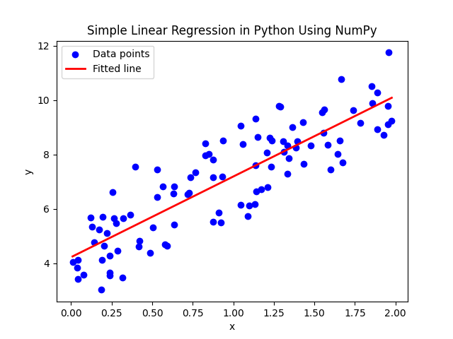
In this Python linear regression example, we:

• Generate synthetic data following a linear relationship.
• Use np.polyfit to Python fit linear regression to the synthetic data, calculating the best-fit parameters.
• Visualize the data and the resulting regression line, illustrating how to do linear regression in Python.

Advanced Curve Fitting Techniques in Python

Beyond linear regression, many real-world problems require modeling non-linear relationships. Python curve fitting capabilities allow you to experiment with various Python regression models to find the best fit for your data. One popular method for non-linear models is using SciPy’s curve_fit method, which helps to find coefficients of custom models.

Example: Quadratic Curve Fitting with SciPy

import numpy as np

import matplotlib.pyplot as plt

from scipy.optimize import curve_fit

# Define the quadratic model function

def quadratic_model(x, a, b, c):

    return a * x**2 + b * x + c

# Generate synthetic data for curve fitting

np.random.seed(0)

x_data = np.linspace(-5, 5, 100)

y_data = quadratic_model(x_data, 2, -3, 5) + np.random.randn(100) * 5

# Fit the quadratic curve using curve_fit

params, covariance = curve_fit(quadratic_model, x_data, y_data)

# Extract the optimal parameters

a_opt, b_opt, c_opt = params

print("Fitted parameters:", params)

# Plot the original data and the fitted curve

plt.scatter(x_data, y_data, label="Data", color="blue")

plt.plot(x_data, quadratic_model(x_data, a_opt, b_opt, c_opt), label="Fitted curve", color="red")

plt.xlabel("x")

plt.ylabel("y")

plt.title("Quadratic Model")

plt.legend()

plt.show()

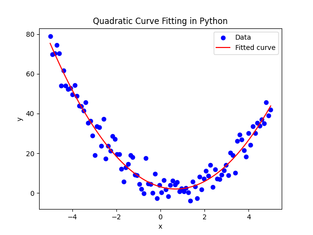
This quadratic fitting example demonstrates how to:

• Define a non-linear model function (a quadratic function).
• Use SciPy’s curve_fit to estimate the best-fit parameters.
• Visualize the original data alongside the fitted curve — showcasing the flexibility of curve_fit method and Python regression models.

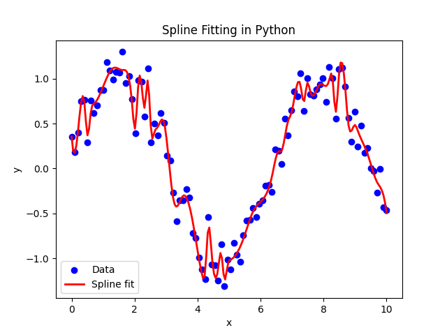
Spline Fitting in Python

Spline fitting is a powerful technique that fits piecewise polynomials to data, ensuring smooth transitions at designated points called knots. This approach is particularly effective when the data exhibits non-linear patterns that a single polynomial function cannot adequately capture.

Python’s SciPy library offers the UnivariateSpline class, which provides a convenient way to perform spline fitting. You can control the smoothness of the resulting curve by adjusting the smoothing factor.

Example: Spline Fitting with SciPy

import numpy as np

import matplotlib.pyplot as plt

from scipy.interpolate import UnivariateSpline

# Generate synthetic data with noise

np.random.seed(0)

x = np.linspace(0, 10, 100)

y = np.sin(x) + np.random.normal(scale=0.2, size=100)

# Fit a univariate spline to the data

spline = UnivariateSpline(x, y, s=1)  # 's' is the smoothing factor

# Generate dense x values for a smooth spline curve

x_dense = np.linspace(0, 10, 200)

y_spline = spline(x_dense)

# Plot the original data and the spline fit

plt.scatter(x, y, label='Data', color='blue')

plt.plot(x_dense, y_spline, label='Spline fit', color='red', linewidth=2)

plt.xlabel('x')

plt.ylabel('y')

plt.title("Spline Fitting in Python")

plt.legend()

plt.show()

In this spline fitting in Python example, we:

• Generate synthetic data that follows a sinusoidal trend with noise.
• Fit a univariate spline using SciPy’s UnivariateSpline.
• Adjust the smoothing factor to balance between closely following the data and achieving a smooth curve.
• Visualize both the original noisy data and the smooth spline fit.

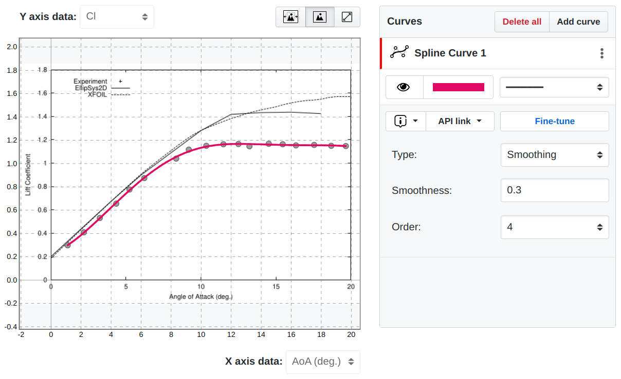
Interactive Curve Fitting and integration with Python

When it comes to interactive curve fitting the best option to choose is SplineCloud.com  —  a web platform with an integrated online spline fitting tool that allows building complex regression models using spline fitting techniques and reusing curves in Python with the help of a client library for Python.

With its intuitive interface, you can adjust parameters — such as knot number, smoothing factor, select different fitting techniques, and much more  —  you can also fine-tune your spline models by adjusting the position of control points and knot vectors. This interactivity not only enhances the user experience but also ensures that the fitted curves closely represent your data’s underlying structure. It is the ultimate tool for building regression models on top of graphical data.

Once you have constructed your curve using SplineCloud’s advanced curve fitting tool, you can seamlessly integrate it into your Python code using the SplineCloud API. This integration allows you to share and reuse the curves, making it straightforward to incorporate complex regression models into code to exclude data loading and processing pipelines, making your code clean and evaluate faster.

Key Benefits of SplineCloud Integration

• Interactive online tool: With SplineCloud’s web interface you can experiment with various fitting parameters in real time. This is particularly useful for building complex models that capture non-linear trends.
• Advanced Curve Fitting: SplineCloud supports parametric splines, making it an excellent choice contrary to traditional curve fitting methods, saving time on data fitting operations and tuning input parameters.
• API Integration: The SplineCloud API lets you retrieve your fitted curves directly from your Python environment. This means you can pull a fitted curve into your code and use it as a regular function without re-fitting the model each time you rerun your code.

Using the SplineCloud API in Python

Below is a basic example of how you might retrieve a fitted curve from SplineCloud and use it in your Python code. But first, you need to install a client library:

pip install splinecloud-scipy

Then, import load_spline method from this library into your code and load your curve using the curve ID that you can copy from the dropdown “API link”

import numpy as np

import matplotlib.pyplot as plt

from splinecloud_scipy import load_spline

curve_id = 'spl_zkGl8Ppw4gPq'

spline = load_spline(curve_id)

X = np.linspace(0, 20, 100)

Y = [spline.eval(x) for x in X]

columns, table = spline.load_data()

x_data, y_data = table.T

plt.plot(X, Y, color='red')

plt.plot(x_data, y_data, 'o', color='blue')

plt.grid()

plt.xlabel(columns[0])

plt.ylabel(columns[1])

plt.show()

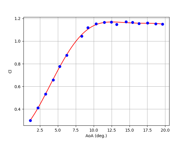
In this example, you use the SplineCloud client library to fetch curve data and reconstruct the function. With this strategy, you can:

• Evaluate the curve against for dependent variable at any point;
• Integrate the model into larger analytical pipelines.
• Update the model parameters interactively if needed, the model will update in the code after re-running it.

Best Practices and Model Evaluation

When performing regression analysis consider these best practices to ensure robust, scalable, and accurate models:

1. Data Preprocessing:
   Ensure your data is thoroughly cleaned — remove outliers, handle missing values, and apply appropriate scaling. Clean data forms the foundation for any reliable model, whether you're performing simple linear fitting or more advanced spline fitting.
2. Model Selection and Complexity:
   If you know that your data exhibits linear trends, begin with simpler models such as linear models using NumPy or SciPy. Alternatively, tools like SplineCloud enable you to experiment with spline configurations, giving you the flexibility to tackle non-linear relationships effectively.
3. Interactive Model Refinement:
   Leverage interactive platforms like SplineCloud to adjust model parameters (e.g., knot placements, smoothing factors) in real time. The SplineCloud client library allows you to easily fetch and integrate updated curves into your Python workflow. This interactivity not only improves model accuracy but also streamlines the process of updating and refining your models.
4. Evaluation Metrics:
   Use statistical metrics such as Mean Squared Error (MSE) and R-squared, alongside residual analysis, to quantitatively assess model performance. Regular evaluation across different model types ensures that you select the most effective regression algorithms for your specific problem.
5. Visualization:
   Plot your original data alongside the fitted curves to visually inspect how well the model captures the underlying trends. Visualization is key, especially when using advanced methods like spline fitting, to confirm that interactive adjustments lead to better data representation.
6. Integration and Scalability:
   Design your workflow so that models can be seamlessly integrated into larger analytical pipelines. The SplineCloud API and its Python client facilitate this integration by allowing you to retrieve and deploy complex curves directly in your code. This ensures your Python regression models are both scalable and maintainable in production environments.
7. Iterative Improvement:
   Continuously refine your models based on feedback from both quantitative metrics and visual inspections. With interactive tools like SplineCloud, updating your model parameters is straightforward — simply re-run your code after adjusting the curve interactively to see immediate improvements in your results.

Following these best practices will help you build robust, accurate, and scalable regression models that fully leverage both traditional curve fitting techniques and modern, interactive platforms like SplineCloud.

Conclusion

This article has provided a comprehensive guide to both linear regression and advanced curve fitting techniques, bridging traditional numerical methods with modern interactive tools. We started by exploring the fundamentals of curve fitting, demonstrating how a linear regression model can be implemented with NumPy for quick and effective analysis. We then expanded into more complex scenarios with non-linear models using SciPy’s curve_fit and flexible, piecewise polynomial approaches with spline fitting in Python.

A key highlight is the integration of interactive tools like SplineCloud. With the SplineCloud client library, you can easily retrieve and reuse fitted curves in your Python environment. This allows for real-time adjustments, enabling you to fine-tune your models and integrate them seamlessly into larger analytical pipelines.

By combining traditional techniques with interactive platforms, you can ensure that your models are accessible and reusable. Whether you're working on a simple linear regression or building advanced regression models that leverage spline fitting, these strategies empower you to optimize your models and confidently address a wide range of data challenges.

Happy coding, and may your models perfectly capture your data’s trends!